library(tidyverse)
library(readxl)
library(skimr)
library(summarytools)
library(patchwork)
library(ggwordcloud)
library(plotly)

date_caption <- "5 janvier 2024"
source("tools/themes.R") # themes

source <- read_csv("posts/2025-01-22/data/antibes_prenoms_naissance_ty62ggz.csv")
df <- sourceIntroduction
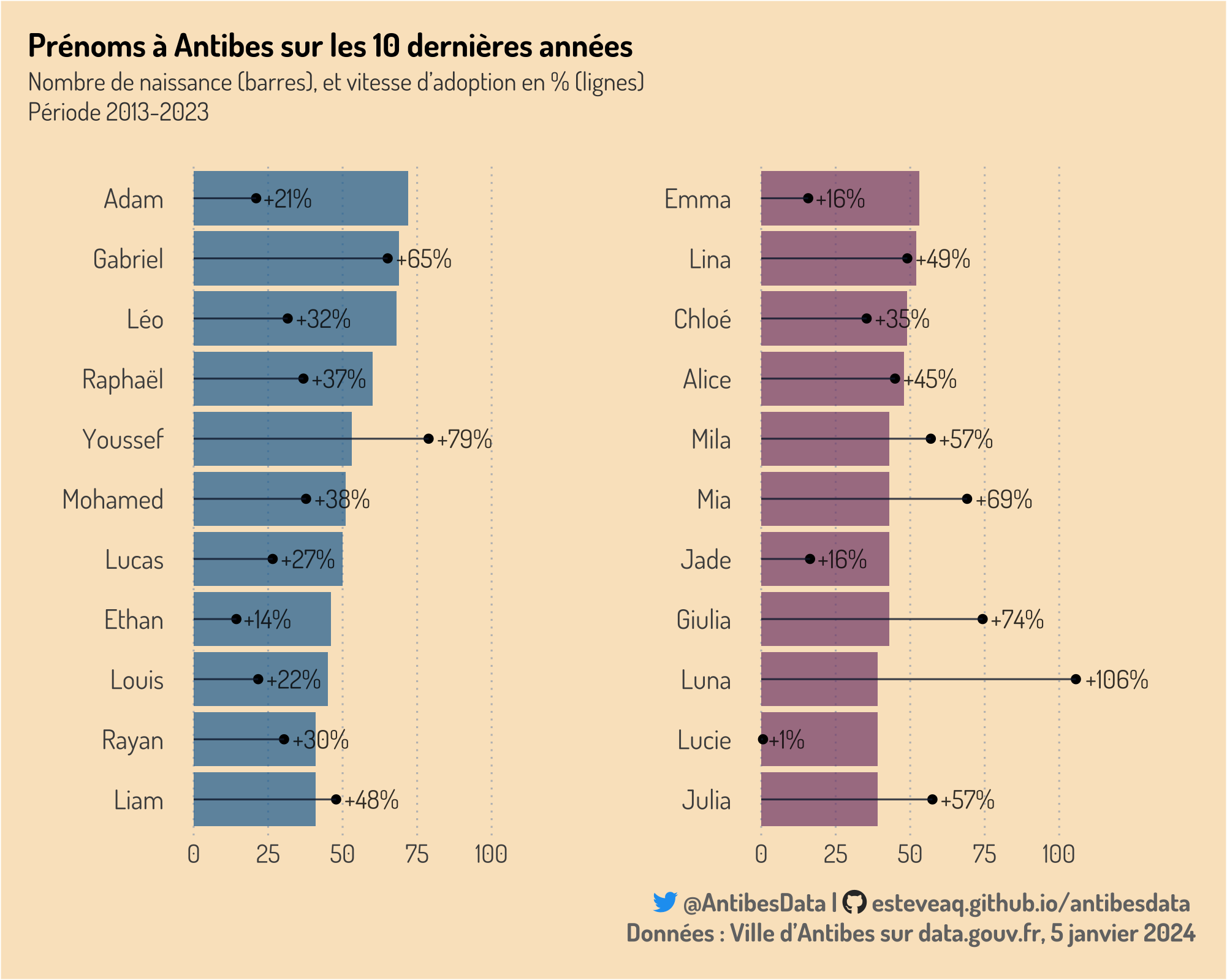
Ce poste propose une analyse statistique des naissances à Antibes Juan-les-Pins sur la période 2013-2023. Un graphe en barres décrit le volume des naissances, et les segments décrivent la croissance moyenne annuelle des prénoms (en %).
Résultats
Au top des prénoms en volume, on trouve Adam pour les garçons avec 72 naissances et Emma pour les filles avec 53 naissances. Au top des prénoms en croissance moyenne annuelle on trouve Youssef (+79%) pour les garçons et Luna (+106%) pour les filles.
Visualisation
Code
Import
Inspect
head(df)
names(df)
glimpse(df)
summary(df)
skim(df)
sapply(df, unique)
dfSummary(df)
Clean
# standardize cols names and variables in chr type
df <-
  df %>%
  rename_with(tolower) %>%
  rename_with(~ str_squish(.)) %>%
  rename_with(~ str_replace_all(., " ", "_")) %>%
  mutate(across(where(is.character), ~ str_squish(str_to_lower(.))))

# remove unwanted cols
df <-
  df %>%
  select(annee, enfant_sexe, enfant_prenom, nombre_occurrences)

# Title case variables
df <-
  df %>%
  mutate(across(c(enfant_sexe, enfant_prenom), str_to_title))

# Filter
df <-
  df %>%
  filter(annee >= 2012)
Analysis
# Evolution of total births
df %>%
    group_by(annee) %>%
    summarize(naissances = sum(nombre_occurrences)) %>% plot(type = "l")
# Top 10
df_top10 <-
  df %>%
  group_by(enfant_sexe, enfant_prenom) %>%
  summarise(n = sum(nombre_occurrences)) %>%
  arrange(-n) %>%
  slice_max(n, n = 10)

# Top 10 Male and Female
  df_top10_M <- df_top10 %>% filter(enfant_sexe == "M")
  df_top10_F <- df_top10 %>% filter(enfant_sexe == "F")

# YoY Growth
dt_prep_yoy <-
  df %>%
    group_by(enfant_prenom) %>%
    mutate(nombre_occurrences_previous = lag(nombre_occurrences, order_by = annee),
           yoy_growth = (nombre_occurrences / nombre_occurrences_previous - 1)*100)

df_yoy <-
dt_prep_yoy %>%
  drop_na() %>%
  group_by(enfant_sexe, enfant_prenom) %>%
  summarise(tot_nombre_occurences = sum(nombre_occurrences), # number of births
            mean_yoy_growth = mean(yoy_growth))      # mean growth rate

df_yoy_top10 <-
df_yoy %>%
  arrange(-tot_nombre_occurences) %>%
  slice_max(tot_nombre_occurences, n = 10) %>%
  filter(enfant_sexe != "I")

df_yoy_top10_M <-
  df_yoy %>%
  filter(enfant_sexe == "M") %>%
  arrange(-tot_nombre_occurences) %>%
  slice_max(tot_nombre_occurences, n = 10)

df_yoy_top10_F <-
  df_yoy %>%
  filter(enfant_sexe == "F") %>%
  arrange(-tot_nombre_occurences) %>%
  slice_max(tot_nombre_occurences, n = 10)
Plot
# Ranking of top 10 names per volume, with adoption rate (Mean YoY Growth)

df_yoy_top10$enfant_sexe <- factor(df_yoy_top10$enfant_sexe, levels = c("M", "F"))

plot_ranking_top10 <-
df_yoy_top10 %>%
 ggplot(aes(x = reorder(enfant_prenom, tot_nombre_occurences), y = tot_nombre_occurences)) +
      geom_bar(aes(fill = enfant_sexe), stat = "identity", alpha = 0.7) +
      geom_point(aes(x =  enfant_prenom, y = mean_yoy_growth), size = 2) +
      geom_segment(aes(
             x = enfant_prenom,
             xend = enfant_prenom,
             y = 0,
             yend = mean_yoy_growth),
         color = darkblue,
         alpha = 0.8,
         size = 0.5) +
      geom_text(aes(
                      x =  enfant_prenom,
                      y = mean_yoy_growth,
                      label = paste0("+", round(mean_yoy_growth, 0), "%")
                    ),
                size = 5,
                hjust = -0.15,
                alpha = 0.8,
                family = setfont
                ) +
  scale_fill_manual(values = c("#1D6FA1", "#824B79")) +
  facet_wrap(~enfant_sexe,  scales = "free_y") +
  scale_y_continuous(limits = c(0,140), breaks = c(0, 25, 50, 75, 100)) +
  coord_flip() + tt7
Render
plot_ranking_top10 +
labs(caption = social_caption2)  +
plot_annotation(
  title = 'Prénoms à Antibes sur les 10 dernières années',
  subtitle = "Nombre de naissance (barres), et vitesse d'adoption en % (lignes) <br>Période 2013-2023",
  theme = theme(
    plot.title = element_text(margin = margin(t = 13, b = 3),
                              hjust = 0,
                              family = setfont,
                              face = "bold",
                              color ="black",
                              size = 18),
    plot.subtitle = element_textbox_simple(
      margin = margin(b = 20),
      hjust = 0,
      family = setfont,
      size = 14,
      colour ="gray25"),
    plot.background = element_rect(fill = "#FAE5C6")
  )
) 
Source
Prénoms des nouveaux-nés à Antibes, disponible sur data.gouv.fr, mise à jour du 5 janvier 2024